
Decision Tree 집값 예측(회귀)
목표
- Decision Tree 모델 사용하기
- 모델 최적화하기
# 예측하기 좋은 최적의 질문을 만들어 학습하는 모델
from sklearn.tree import DecisionTreeRegressor

house_model = DecisionTreeRegressor()
2. 모델 학습
- 데이터 로딩 후 탐색
import pandas as pd

# 데이터 로딩
train = pd.read_csv('./data/house/train.csv')
test = pd.read_csv('./data/house/test.csv')
train.head()
| Id | Suburb | Address | Rooms | Type | Method | SellerG | Date | Distance | Postcode | … | Car | Landsize | BuildingArea | YearBuilt | CouncilArea | Lattitude | Longtitude | Regionname | Propertycount | Price | |
|---|---|---|---|---|---|---|---|---|---|---|---|---|---|---|---|---|---|---|---|---|---|
| 0 | 5467 | Rosanna | 22 Douglas St | 2 | h | S | Miles | 19/11/2016 | 11.4 | 3084 | … | 1.0 | 757 | NaN | NaN | Banyule | -37.74280 | 145.07000 | Eastern Metropolitan | 3540 | 1200000 |
| 1 | 4365 | North Melbourne | 103/25 Byron St | 1 | u | SP | Jellis | 16/07/2016 | 2.3 | 3051 | … | 1.0 | 0 | 60.0 | 2012.0 | Melbourne | -37.80200 | 144.95160 | Northern Metropolitan | 6821 | 450000 |
| 2 | 9741 | Surrey Hills | 4/40 Durham Rd | 3 | u | SP | Noel | 17/06/2017 | 10.2 | 3127 | … | 1.0 | 149 | NaN | NaN | Boroondara | -37.82971 | 145.09007 | Southern Metropolitan | 5457 | 780000 |
| 3 | 11945 | Cheltenham | 3/33 Sunray Av | 2 | t | S | Buxton | 29/07/2017 | 17.9 | 3192 | … | 1.0 | 171 | NaN | NaN | Kingston | -37.96304 | 145.06421 | Southern Metropolitan | 9758 | 751000 |
| 4 | 4038 | Mont Albert | 7/27 High St | 3 | t | S | Fletchers | 15/10/2016 | 11.8 | 3127 | … | 2.0 | 330 | 148.0 | 2001.0 | Whitehorse | -37.81670 | 145.10700 | Eastern Metropolitan | 2079 | 1310000 |
5 rows × 22 columns
# 전체 데이터 갯수 파악
train.shape, test.shape
((10185, 22), (3395, 21))
# 컬럼 확인
train.info()
<class 'pandas.core.frame.DataFrame'>
RangeIndex: 10185 entries, 0 to 10184
Data columns (total 22 columns):
 #   Column         Non-Null Count  Dtype
---  ------         --------------  -----
 0   Id             10185 non-null  int64
 1   Suburb         10185 non-null  object
 2   Address        10185 non-null  object
 3   Rooms          10185 non-null  int64
 4   Type           10185 non-null  object
 5   Method         10185 non-null  object
 6   SellerG        10185 non-null  object
 7   Date           10185 non-null  object
 8   Distance       10185 non-null  float64
 9   Postcode       10185 non-null  int64
 10  Bedroom2       10185 non-null  int64
 11  Bathroom       10185 non-null  int64
 12  Car            10142 non-null  float64
 13  Landsize       10185 non-null  int64
 14  BuildingArea   5367 non-null   float64
 15  YearBuilt      6153 non-null   float64
 16  CouncilArea    9174 non-null   object
 17  Lattitude      10185 non-null  float64
 18  Longtitude     10185 non-null  float64
 19  Regionname     10185 non-null  object
 20  Propertycount  10185 non-null  int64
 21  Price          10185 non-null  int64
dtypes: float64(6), int64(8), object(8)
memory usage: 1.7+ MB
# 기술 통계, include='all' 범주형 통계 값 포함(고유값, 최빈값, ...)
train.describe(include='all')
| Id | Suburb | Address | Rooms | Type | Method | SellerG | Date | Distance | Postcode | … | Car | Landsize | BuildingArea | YearBuilt | CouncilArea | Lattitude | Longtitude | Regionname | Propertycount | Price | |
|---|---|---|---|---|---|---|---|---|---|---|---|---|---|---|---|---|---|---|---|---|---|
| count | 10185.000000 | 10185 | 10185 | 10185.000000 | 10185 | 10185 | 10185 | 10185 | 10185.000000 | 10185.000000 | … | 10142.000000 | 10185.000000 | 5367.000000 | 6153.000000 | 9174 | 10185.000000 | 10185.000000 | 10185 | 10185.000000 | 1.018500e+04 |
| unique | NaN | 310 | 10066 | NaN | 3 | 5 | 243 | 58 | NaN | NaN | … | NaN | NaN | NaN | NaN | 33 | NaN | NaN | 8 | NaN | NaN |
| top | NaN | Reservoir | 2 Bruce St | NaN | h | S | Nelson | 27/05/2017 | NaN | NaN | … | NaN | NaN | NaN | NaN | Moreland | NaN | NaN | Southern Metropolitan | NaN | NaN |
| freq | NaN | 261 | 3 | NaN | 7106 | 6753 | 1156 | 364 | NaN | NaN | … | NaN | NaN | NaN | NaN | 887 | NaN | NaN | 3525 | NaN | NaN |
| mean | 6802.613942 | NaN | NaN | 2.943250 | NaN | NaN | NaN | NaN | 10.198213 | 3105.172607 | … | 1.613883 | 573.426411 | 154.137372 | 1964.904599 | NaN | -37.809763 | 144.995347 | NaN | 7447.172018 | 1.077961e+06 |
| std | 3926.702100 | NaN | NaN | 0.952794 | NaN | NaN | NaN | NaN | 5.866640 | 90.198740 | … | 0.959076 | 4550.757180 | 614.711880 | 37.603561 | NaN | 0.079922 | 0.104255 | NaN | 4354.473015 | 6.364301e+05 |
| min | 3.000000 | NaN | NaN | 1.000000 | NaN | NaN | NaN | NaN | 0.000000 | 3000.000000 | … | 0.000000 | 0.000000 | 0.000000 | 1196.000000 | NaN | -38.182550 | 144.431810 | NaN | 249.000000 | 1.310000e+05 |
| 25% | 3384.000000 | NaN | NaN | 2.000000 | NaN | NaN | NaN | NaN | 6.200000 | 3044.000000 | … | 1.000000 | 178.000000 | 93.920000 | 1940.000000 | NaN | -37.857700 | 144.929500 | NaN | 4380.000000 | 6.500000e+05 |
| 50% | 6838.000000 | NaN | NaN | 3.000000 | NaN | NaN | NaN | NaN | 9.300000 | 3084.000000 | … | 2.000000 | 448.000000 | 127.000000 | 1970.000000 | NaN | -37.802900 | 145.000130 | NaN | 6543.000000 | 9.050000e+05 |
| 75% | 10223.000000 | NaN | NaN | 4.000000 | NaN | NaN | NaN | NaN | 13.000000 | 3149.000000 | … | 2.000000 | 652.000000 | 175.000000 | 2000.000000 | NaN | -37.756710 | 145.059280 | NaN | 10331.000000 | 1.330000e+06 |
| max | 13577.000000 | NaN | NaN | 8.000000 | NaN | NaN | NaN | NaN | 48.100000 | 3977.000000 | … | 10.000000 | 433014.000000 | 44515.000000 | 2018.000000 | NaN | -37.408530 | 145.526350 | NaN | 21650.000000 | 7.650000e+06 |
11 rows × 22 columns
- 문제와 정답 추출
- 일단은 결측치가 존재하는 컬럼과 문자형태의 컬럼은 배제
X_train = train[['Propertycount', 'Rooms', 'Bedroom2']]
y_train = train['Price']
# train -> 7.5 : 2.5비율로 train2, validation 데이터로 나누기
from sklearn.model_selection import train_test_split

X_train2, X_val, y_train2, y_val = train_test_split(X_train, y_train, random_state=3)
X_train2.shape, X_val.shape, y_train2.shape, y_val.shape
((7638, 3), (2547, 3), (7638,), (2547,))
house_model.fit(X_train2, y_train2)
DecisionTreeRegressor()
3. 모델 예측
pred = house_model.predict(X_val)
pred
array([ 451840. , 1344925. , 684462.5, …, 1843500. , 1300000. , 2272500. ])
4. 모델 평가
- MAE(Mean Absolute Error, 평균 절대값 오차) 활용한 평가
from sklearn.metrics import mean_absolute_error
error = mean_absolute_error(y_val, pred)
error
255227.3455560717
캐글에 업로드 하기
X_test = test[['Propertycount', 'Rooms', 'Bedroom2']]
X_test.shape
(3395, 3)
test_pre = house_model.predict(X_test)
test_pre
array([ 382333.33333333, 522500. , 700000. , …, 710500. , 651357.14285714, 1042205.88235294])
# 정답지 파일 로딩
submission = pd.read_csv("./data/house/sample_submission.csv")
submission
| Id | Price | |
|---|---|---|
| 0 | 3189 | 0 |
| 1 | 2539 | 0 |
| 2 | 9171 | 0 |
| 3 | 4741 | 0 |
| 4 | 12455 | 0 |
| … | … | … |
| 3390 | 12276 | 0 |
| 3391 | 4618 | 0 |
| 3392 | 12913 | 0 |
| 3393 | 11741 | 0 |
| 3394 | 1072 | 0 |
3395 rows × 2 columns
test.head()
| Id | Suburb | Address | Rooms | Type | Method | SellerG | Date | Distance | Postcode | … | Bathroom | Car | Landsize | BuildingArea | YearBuilt | CouncilArea | Lattitude | Longtitude | Regionname | Propertycount | |
|---|---|---|---|---|---|---|---|---|---|---|---|---|---|---|---|---|---|---|---|---|---|
| 0 | 3189 | Hawthorn | 22/9 Lisson Gr | 1 | u | S | Biggin | 19/11/2016 | 4.6 | 3122 | … | 1 | 1.0 | 0 | 52.0 | 1970.0 | Boroondara | -37.82610 | 145.02690 | Southern Metropolitan | 11308 |
| 1 | 2539 | Fitzroy | 113/300 Young St | 1 | u | SP | Jellis | 19/11/2016 | 1.6 | 3065 | … | 1 | 1.0 | 0 | 52.0 | 2011.0 | Yarra | -37.79740 | 144.97990 | Northern Metropolitan | 5825 |
| 2 | 9171 | Greenvale | 7 Murray Ct | 5 | h | S | Barry | 3/06/2017 | 20.4 | 3059 | … | 3 | 5.0 | 1750 | 310.0 | 1990.0 | Hume | -37.65439 | 144.89113 | Northern Metropolitan | 4864 |
| 3 | 4741 | Port Melbourne | 172 Albert St | 2 | h | S | hockingstuart | 10/12/2016 | 3.8 | 3207 | … | 1 | 0.0 | 106 | 70.0 | 1910.0 | Port Phillip | -37.83460 | 144.93730 | Southern Metropolitan | 8648 |
| 4 | 12455 | Brunswick West | 47 Everett St | 4 | h | VB | Nelson | 9/09/2017 | 5.2 | 3055 | … | 2 | 2.0 | 600 | 180.0 | 2004.0 | NaN | -37.75465 | 144.94144 | Northern Metropolitan | 7082 |
5 rows × 21 columns
submission['Price'] = test_pre
submission.head()
| Id | Price | |
|---|---|---|
| 0 | 3189 | 3.823333e+05 |
| 1 | 2539 | 5.225000e+05 |
| 2 | 9171 | 7.000000e+05 |
| 3 | 4741 | 9.572778e+05 |
| 4 | 12455 | 1.294818e+06 |
# csv파일로 저장
submission.to_csv("./data/house/myPrediction.csv",
                 index=False)
다른 컬럼을 이용해보자.
- 결측치가 있는 컬럼
- 데이터를 버린다. -> drop, dropna
- 데이터를 채운다. -> fillna
- 기술통계 활용
- 모델 활용 -> 결측치를 정답, 주변컬럼을 문제로 설정
- 문자형태의 컬럼
- 문자타입 -> 숫자타입 변경(인코딩)
- 라벨 인코딩 -> 임의의 숫자를 글자에 부여
- 원핫 인코딩 -> 0과1을 이용해서 변환
- 문자타입 -> 숫자타입 변경(인코딩)
test.columns
Index([‘Id’, ‘Suburb’, ‘Address’, ‘Rooms’, ‘Type’, ‘Method’, ‘SellerG’, ‘Date’, ‘Distance’, ‘Postcode’, ‘Bedroom2’, ‘Bathroom’, ‘Car’, ‘Landsize’, ‘BuildingArea’, ‘YearBuilt’, ‘CouncilArea’, ‘Lattitude’, ‘Longtitude’, ‘Regionname’, ‘Propertycount’], dtype=‘object’)
train.corr()
| | Id | Rooms | Distance | Postcode | Bedroom2 | Bathroom | Car | Landsize | BuildingArea | YearBuilt | Lattitude | Longtitude | Propertycount | Price | h | t | u | Method_label | Regionname_label | | — | — | — | — | — | — | — | — | — | — | — | — | — | — | — | — | — | — | — | — | | Id | 1.000000 | 0.100741 | 0.293943 | 0.092843 | 0.116731 | 0.040834 | 0.099056 | 0.026959 | 0.024208 | 0.104456 | 0.040772 | 0.056133 | 0.008075 | -0.051498 | 0.114506 | -0.041921 | -0.099133 | 0.011529 | 0.267904 | | Rooms | 0.100741 | 1.000000 | 0.294621 | 0.053791 | 0.937357 | 0.588991 | 0.406340 | 0.024508 | 0.115067 | -0.059154 | 0.012710 | 0.104277 | -0.081669 | 0.497539 | 0.507407 | -0.028028 | -0.543692 | 0.003428 | 0.166209 | | Distance | 0.293943 | 0.294621 | 1.000000 | 0.430208 | 0.294438 | 0.120574 | 0.268467 | 0.024602 | 0.108834 | 0.245371 | -0.134113 | 0.239075 | -0.052206 | -0.164388 | 0.213490 | -0.012074 | -0.228571 | -0.093669 | 0.510509 | | Postcode | 0.092843 | 0.053791 | 0.430208 | 1.000000 | 0.059840 | 0.108927 | 0.052475 | 0.027304 | 0.061235 | 0.021593 | -0.408562 | 0.450340 | 0.057250 | 0.111511 | -0.024155 | -0.008960 | 0.032696 | 0.016300 | -0.055349 | | Bedroom2 | 0.116731 | 0.937357 | 0.294438 | 0.059840 | 1.000000 | 0.579122 | 0.402223 | 0.024382 | 0.112563 | -0.045148 | 0.012189 | 0.105248 | -0.080096 | 0.473742 | 0.485838 | -0.027327 | -0.520256 | 0.005557 | 0.165695 | | Bathroom | 0.040834 | 0.588991 | 0.120574 | 0.108927 | 0.579122 | 1.000000 | 0.319449 | 0.038824 | 0.106673 | 0.154065 | -0.072667 | 0.116156 | -0.050214 | 0.464396 | 0.169435 | 0.119998 | -0.267174 | 0.084622 | 0.015280 | | Car | 0.099056 | 0.406340 | 0.268467 | 0.052475 | 0.402223 | 0.319449 | 1.000000 | 0.023537 | 0.096233 | 0.113786 | -0.003670 | 0.067147 | -0.024338 | 0.235853 | 0.253054 | -0.014562 | -0.270764 | 0.012097 | 0.112987 | | Landsize | 0.026959 | 0.024508 | 0.024602 | 0.027304 | 0.024382 | 0.038824 | 0.023537 | 1.000000 | 0.546089 | 0.040293 | 0.010407 | 0.010326 | -0.009704 | 0.040665 | 0.022618 | -0.018688 | -0.012693 | 0.029722 | 0.022445 | | BuildingArea | 0.024208 | 0.115067 | 0.108834 | 0.061235 | 0.112563 | 0.106673 | 0.096233 | 0.546089 | 1.000000 | 0.021732 | 0.052281 | -0.033764 | -0.029216 | 0.082028 | 0.060088 | -0.004645 | -0.064177 | -0.001155 | 0.060186 | | YearBuilt | 0.104456 | -0.059154 | 0.245371 | 0.021593 | -0.045148 | 0.154065 | 0.113786 | 0.040293 | 0.021732 | 1.000000 | 0.060937 | -0.017734 | 0.006838 | -0.324162 | -0.393885 | 0.298914 | 0.230626 | 0.027549 | 0.130729 | | Lattitude | 0.040772 | 0.012710 | -0.134113 | -0.408562 | 0.012189 | -0.072667 | -0.003670 | 0.010407 | 0.052281 | 0.060937 | 1.000000 | -0.359648 | 0.060830 | -0.210428 | 0.108648 | -0.035545 | -0.096862 | -0.027790 | 0.141548 | | Longtitude | 0.056133 | 0.104277 | 0.239075 | 0.450340 | 0.105248 | 0.116156 | 0.067147 | 0.010326 | -0.033764 | -0.017734 | -0.359648 | 1.000000 | 0.056610 | 0.206866 | -0.008365 | 0.006092 | 0.005237 | 0.022174 | -0.006846 | | Propertycount | 0.008075 | -0.081669 | -0.052206 | 0.057250 | -0.080096 | -0.050214 | -0.024338 | -0.009704 | -0.029216 | 0.006838 | 0.060830 | 0.056610 | 1.000000 | -0.046582 | -0.065180 | -0.020591 | 0.085853 | -0.005943 | -0.184688 | | Price | -0.051498 | 0.497539 | -0.164388 | 0.111511 | 0.473742 | 0.464396 | 0.235853 | 0.040665 | 0.082028 | -0.324162 | -0.210428 | 0.206866 | -0.046582 | 1.000000 | 0.391641 | -0.061995 | -0.392931 | 0.029182 | -0.237278 | | h | 0.114506 | 0.507407 | 0.213490 | -0.024155 | 0.485838 | 0.169435 | 0.253054 | 0.022618 | 0.060088 | -0.393885 | 0.108648 | -0.008365 | -0.065180 | 0.391641 | 1.000000 | -0.453989 | -0.807573 | -0.065250 | 0.191063 | | t | -0.041921 | -0.028028 | -0.012074 | -0.008960 | -0.027327 | 0.119998 | -0.014562 | -0.018688 | -0.004645 | 0.298914 | -0.035545 | 0.006092 | -0.020591 | -0.061995 | -0.453989 | 1.000000 | -0.158859 | 0.008709 | -0.037968 | | u | -0.099133 | -0.543692 | -0.228571 | 0.032696 | -0.520256 | -0.267174 | -0.270764 | -0.012693 | -0.064177 | 0.230626 | -0.096862 | 0.005237 | 0.085853 | -0.392931 | -0.807573 | -0.158859 | 1.000000 | 0.066537 | -0.186580 | | Method_label | 0.011529 | 0.003428 | -0.093669 | 0.016300 | 0.005557 | 0.084622 | 0.012097 | 0.029722 | -0.001155 | 0.027549 | -0.027790 | 0.022174 | -0.005943 | 0.029182 | -0.065250 | 0.008709 | 0.066537 | 1.000000 | -0.070270 | | Regionname_label | 0.267904 | 0.166209 | 0.510509 | -0.055349 | 0.165695 | 0.015280 | 0.112987 | 0.022445 | 0.060186 | 0.130729 | 0.141548 | -0.006846 | -0.184688 | -0.237278 | 0.191063 | -0.037968 | -0.186580 | -0.070270 | 1.000000 |
- Type 컬럼 전처리
# 원한인코딩 함수
type_onehot = pd.get_dummies(train['Type'])
type_onehot
| h | t | u | |
|---|---|---|---|
| 0 | 1 | 0 | 0 |
| 1 | 0 | 0 | 1 |
| 2 | 0 | 0 | 1 |
| 3 | 0 | 1 | 0 |
| 4 | 0 | 1 | 0 |
| … | … | … | … |
| 10180 | 1 | 0 | 0 |
| 10181 | 1 | 0 | 0 |
| 10182 | 1 | 0 | 0 |
| 10183 | 1 | 0 | 0 |
| 10184 | 0 | 1 | 0 |
10185 rows × 3 columns
type_onehot_test = pd.get_dummies(test['Type'])
type_onehot_test
| h | t | u | |
|---|---|---|---|
| 0 | 0 | 0 | 1 |
| 1 | 0 | 0 | 1 |
| 2 | 1 | 0 | 0 |
| 3 | 1 | 0 | 0 |
| 4 | 1 | 0 | 0 |
| … | … | … | … |
| 3390 | 1 | 0 | 0 |
| 3391 | 1 | 0 | 0 |
| 3392 | 0 | 1 | 0 |
| 3393 | 1 | 0 | 0 |
| 3394 | 0 | 0 | 1 |
3395 rows × 3 columns
train = pd.concat([train, type_onehot], axis=1)
train.head()
| Id | Suburb | Address | Rooms | Type | Method | SellerG | Date | Distance | Postcode | … | YearBuilt | CouncilArea | Lattitude | Longtitude | Regionname | Propertycount | Price | h | t | u | |
|---|---|---|---|---|---|---|---|---|---|---|---|---|---|---|---|---|---|---|---|---|---|
| 0 | 5467 | Rosanna | 22 Douglas St | 2 | h | S | Miles | 19/11/2016 | 11.4 | 3084 | … | NaN | Banyule | -37.74280 | 145.07000 | Eastern Metropolitan | 3540 | 1200000 | 1 | 0 | 0 |
| 1 | 4365 | North Melbourne | 103/25 Byron St | 1 | u | SP | Jellis | 16/07/2016 | 2.3 | 3051 | … | 2012.0 | Melbourne | -37.80200 | 144.95160 | Northern Metropolitan | 6821 | 450000 | 0 | 0 | 1 |
| 2 | 9741 | Surrey Hills | 4/40 Durham Rd | 3 | u | SP | Noel | 17/06/2017 | 10.2 | 3127 | … | NaN | Boroondara | -37.82971 | 145.09007 | Southern Metropolitan | 5457 | 780000 | 0 | 0 | 1 |
| 3 | 11945 | Cheltenham | 3/33 Sunray Av | 2 | t | S | Buxton | 29/07/2017 | 17.9 | 3192 | … | NaN | Kingston | -37.96304 | 145.06421 | Southern Metropolitan | 9758 | 751000 | 0 | 1 | 0 |
| 4 | 4038 | Mont Albert | 7/27 High St | 3 | t | S | Fletchers | 15/10/2016 | 11.8 | 3127 | … | 2001.0 | Whitehorse | -37.81670 | 145.10700 | Eastern Metropolitan | 2079 | 1310000 | 0 | 1 | 0 |
5 rows × 25 columns
test = pd.concat([test, type_onehot_test], axis=1)
test.head()
| Id | Suburb | Address | Rooms | Type | Method | SellerG | Date | Distance | Postcode | … | BuildingArea | YearBuilt | CouncilArea | Lattitude | Longtitude | Regionname | Propertycount | h | t | u | |
|---|---|---|---|---|---|---|---|---|---|---|---|---|---|---|---|---|---|---|---|---|---|
| 0 | 3189 | Hawthorn | 22/9 Lisson Gr | 1 | u | S | Biggin | 19/11/2016 | 4.6 | 3122 | … | 52.0 | 1970.0 | Boroondara | -37.82610 | 145.02690 | Southern Metropolitan | 11308 | 0 | 0 | 1 |
| 1 | 2539 | Fitzroy | 113/300 Young St | 1 | u | SP | Jellis | 19/11/2016 | 1.6 | 3065 | … | 52.0 | 2011.0 | Yarra | -37.79740 | 144.97990 | Northern Metropolitan | 5825 | 0 | 0 | 1 |
| 2 | 9171 | Greenvale | 7 Murray Ct | 5 | h | S | Barry | 3/06/2017 | 20.4 | 3059 | … | 310.0 | 1990.0 | Hume | -37.65439 | 144.89113 | Northern Metropolitan | 4864 | 1 | 0 | 0 |
| 3 | 4741 | Port Melbourne | 172 Albert St | 2 | h | S | hockingstuart | 10/12/2016 | 3.8 | 3207 | … | 70.0 | 1910.0 | Port Phillip | -37.83460 | 144.93730 | Southern Metropolitan | 8648 | 1 | 0 | 0 |
| 4 | 12455 | Brunswick West | 47 Everett St | 4 | h | VB | Nelson | 9/09/2017 | 5.2 | 3055 | … | 180.0 | 2004.0 | NaN | -37.75465 | 144.94144 | Northern Metropolitan | 7082 | 1 | 0 | 0 |
5 rows × 24 columns
- Method 컬럼 전처리
# 라벨인코딩
# 캐글의 metadata 정보 참고
method_dict = {
    'S' : 0,
    'SP' : 1,
    'PI' : 2,
    'PN' : 3,
    'SN' : 4,
    'NB' : 5,
    'VB' : 6,
    'W' : 7,
    'SA' : 8,
    'SS' : 9
}
method_label = train['Method'].map(method_dict)
method_label_test = test['Method'].map(method_dict)
method_label
0        0
1        1
2        1
3        0
4        0
        ..
10180    0
10181    2
10182    0
10183    2
10184    0
Name: Method, Length: 10185, dtype: int64
train['Method_label'] = method_label
test['Method_label'] = method_label_test
train.head()
| Id | Suburb | Address | Rooms | Type | Method | SellerG | Date | Distance | Postcode | … | CouncilArea | Lattitude | Longtitude | Regionname | Propertycount | Price | h | t | u | Method_label | |
|---|---|---|---|---|---|---|---|---|---|---|---|---|---|---|---|---|---|---|---|---|---|
| 0 | 5467 | Rosanna | 22 Douglas St | 2 | h | S | Miles | 19/11/2016 | 11.4 | 3084 | … | Banyule | -37.74280 | 145.07000 | Eastern Metropolitan | 3540 | 1200000 | 1 | 0 | 0 | 0 |
| 1 | 4365 | North Melbourne | 103/25 Byron St | 1 | u | SP | Jellis | 16/07/2016 | 2.3 | 3051 | … | Melbourne | -37.80200 | 144.95160 | Northern Metropolitan | 6821 | 450000 | 0 | 0 | 1 | 1 |
| 2 | 9741 | Surrey Hills | 4/40 Durham Rd | 3 | u | SP | Noel | 17/06/2017 | 10.2 | 3127 | … | Boroondara | -37.82971 | 145.09007 | Southern Metropolitan | 5457 | 780000 | 0 | 0 | 1 | 1 |
| 3 | 11945 | Cheltenham | 3/33 Sunray Av | 2 | t | S | Buxton | 29/07/2017 | 17.9 | 3192 | … | Kingston | -37.96304 | 145.06421 | Southern Metropolitan | 9758 | 751000 | 0 | 1 | 0 | 0 |
| 4 | 4038 | Mont Albert | 7/27 High St | 3 | t | S | Fletchers | 15/10/2016 | 11.8 | 3127 | … | Whitehorse | -37.81670 | 145.10700 | Eastern Metropolitan | 2079 | 1310000 | 0 | 1 | 0 | 0 |
5 rows × 26 columns
결측치와 문자형태를 처리해서 다양한 컬럼으로 학습해보자.
- train, test 데이터에 원하는 결측치,인코딩 처리 실시
- 원하는 컬럼 선택
- train을 train2와 val로 분리
- 모델 학습 후 평가
- test 데이터를 예측해 kaggle에 업로드
- Car 컬럼 전처리
# Car 컬럼의 결측치 채우기
train['Car'].describe()
count    10142.000000
mean         1.613883
std          0.959076
min          0.000000
25%          1.000000
50%          2.000000
75%          2.000000
max         10.000000
Name: Car, dtype: float64
# 중앙값으로 채우기
train['Car'] = train['Car'].fillna(train['Car'].median())
test['Car'] = test['Car'].fillna(train['Car'].median())
- Regionname 컬럼 전처리
train['Regionname'].value_counts()
Southern Metropolitan         3525
Northern Metropolitan         2912
Western Metropolitan          2219
Eastern Metropolitan          1096
South-Eastern Metropolitan     348
Eastern Victoria                37
Northern Victoria               30
Western Victoria                18
Name: Regionname, dtype: int64
regionname_dict = {
    'Southern Metropolitan' : 0,
    'Northern Metropolitan' : 1,
    'Western Metropolitan' : 2,
    'Eastern Metropolitan' : 3,
    'South-Eastern Metropolitan' : 4,
    'Eastern Victoria' : 5,
    'Northern Victoria' : 6,
    'Western Victoria' : 7
}

regionname_label = train['Regionname'].map(regionname_dict)
regionname_label_test = test['Regionname'].map(regionname_dict)
regionname_label
train['Regionname_label'] = regionname_label
test['Regionname_label'] = regionname_label_test
train.head()
| Id | Suburb | Address | Rooms | Type | Method | SellerG | Date | Distance | Postcode | … | Lattitude | Longtitude | Regionname | Propertycount | Price | h | t | u | Method_label | Regionname_label | |
|---|---|---|---|---|---|---|---|---|---|---|---|---|---|---|---|---|---|---|---|---|---|
| 0 | 5467 | Rosanna | 22 Douglas St | 2 | h | S | Miles | 19/11/2016 | 11.4 | 3084 | … | -37.74280 | 145.07000 | Eastern Metropolitan | 3540 | 1200000 | 1 | 0 | 0 | 0 | 3 |
| 1 | 4365 | North Melbourne | 103/25 Byron St | 1 | u | SP | Jellis | 16/07/2016 | 2.3 | 3051 | … | -37.80200 | 144.95160 | Northern Metropolitan | 6821 | 450000 | 0 | 0 | 1 | 1 | 1 |
| 2 | 9741 | Surrey Hills | 4/40 Durham Rd | 3 | u | SP | Noel | 17/06/2017 | 10.2 | 3127 | … | -37.82971 | 145.09007 | Southern Metropolitan | 5457 | 780000 | 0 | 0 | 1 | 1 | 0 |
| 3 | 11945 | Cheltenham | 3/33 Sunray Av | 2 | t | S | Buxton | 29/07/2017 | 17.9 | 3192 | … | -37.96304 | 145.06421 | Southern Metropolitan | 9758 | 751000 | 0 | 1 | 0 | 0 | 0 |
| 4 | 4038 | Mont Albert | 7/27 High St | 3 | t | S | Fletchers | 15/10/2016 | 11.8 | 3127 | … | -37.81670 | 145.10700 | Eastern Metropolitan | 2079 | 1310000 | 0 | 1 | 0 | 0 | 3 |
5 rows × 27 columns
- CouncilArea 전처리
X_train = train[['Rooms', 'Distance', 'Bedroom2', 'Bathroom', 'Car', 'Landsize', 'Propertycount', 'h', 't', 'u', 'Method_label', 'Regionname_label', 'Lattitude', 'Longtitude']]
y_train = train['Price']

X_test = test[['Rooms', 'Distance', 'Bedroom2', 'Bathroom', 'Car', 'Landsize', 'Propertycount', 'h', 't', 'u', 'Method_label', 'Regionname_label', 'Lattitude', 'Longtitude']]
X_train.head()
| Rooms | Distance | Bedroom2 | Bathroom | Car | Landsize | Propertycount | h | t | u | Method_label | Regionname_label | Lattitude | Longtitude | |
|---|---|---|---|---|---|---|---|---|---|---|---|---|---|---|
| 0 | 2 | 11.4 | 2 | 1 | 1.0 | 757 | 3540 | 1 | 0 | 0 | 0 | 3 | -37.74280 | 145.07000 |
| 1 | 1 | 2.3 | 1 | 1 | 1.0 | 0 | 6821 | 0 | 0 | 1 | 1 | 1 | -37.80200 | 144.95160 |
| 2 | 3 | 10.2 | 2 | 1 | 1.0 | 149 | 5457 | 0 | 0 | 1 | 1 | 0 | -37.82971 | 145.09007 |
| 3 | 2 | 17.9 | 2 | 1 | 1.0 | 171 | 9758 | 0 | 1 | 0 | 0 | 0 | -37.96304 | 145.06421 |
| 4 | 3 | 11.8 | 3 | 2 | 2.0 | 330 | 2079 | 0 | 1 | 0 | 0 | 3 | -37.81670 | 145.10700 |
X_test.head()
| | Rooms | Distance | Bedroom2 | Bathroom | Car | Landsize | Propertycount | h | t | u | Method_label | Regionname_label | Lattitude | Longtitude | | — | — | — | — | — | — | — | — | — | — | — | — | — | — | — | | 0 | 1 | 4.6 | 1 | 1 | 1.0 | 0 | 11308 | 0 | 0 | 1 | 0 | 0 | -37.82610 | 145.02690 | | 1 | 1 | 1.6 | 1 | 1 | 1.0 | 0 | 5825 | 0 | 0 | 1 | 1 | 1 | -37.79740 | 144.97990 | | 2 | 5 | 20.4 | 5 | 3 | 5.0 | 1750 | 4864 | 1 | 0 | 0 | 0 | 1 | -37.65439 | 144.89113 | | 3 | 2 | 3.8 | 2 | 1 | 0.0 | 106 | 8648 | 1 | 0 | 0 | 0 | 0 | -37.83460 | 144.93730 | | 4 | 4 | 5.2 | 4 | 2 | 2.0 | 600 | 7082 | 1 | 0 | 0 | 6 | 1 | -37.75465 | 144.94144 |
- 검증데이터 분리
X_train3, X_val3, y_train3, y_val3 = train_test_split(X_train, y_train, test_size=0.2, random_state=916)
- 모델 정의
house_model2 = DecisionTreeRegressor()
- 모델 학습
house_model2.fit(X_train3, y_train3)
DecisionTreeRegressor()
- 모델 예측
pred = house_model2.predict(X_val3)
- 모델 평가
mean_absolute_error(y_val3, pred)
245946.3264604811
- 캐글 제출
submission['Price'] = house_model2.predict(X_test)
submission.head()
| Id | Price | |
|---|---|---|
| 0 | 3189 | 348000.0 |
| 1 | 2539 | 597000.0 |
| 2 | 9171 | 725500.0 |
| 3 | 4741 | 1000000.0 |
| 4 | 12455 | 1610000.0 |
submission.to_csv("./data/house/myPrediction.csv",
                 index=False)
모델 최적화
- 모델복잡도 제어하기
- KNN은 이웃의 숫자로 모델의 복잡도 제어
- 이웃의 숫자가 커질수록 단순,
- 숫자가 적어질수록 복잡해진다.
- DecisionTree는 질문의 깊이로 모델의 복잡도를 제어(max_depth)
- 깊이가 얕으면 단순,
- 깊이가 깊으면 복잡해진다.
train_score_list = []
val_score_list = []

for d in range(1, 30):
    m = DecisionTreeRegressor(max_depth=d)
    m.fit(X_train3, y_train3)
    pred_train = m.predict(X_train3)
    pred_val = m.predict(X_val3)

    score_train = mean_absolute_error(y_train3, pred_train)
    score_val = mean_absolute_error(y_val3, pred_val)
    train_score_list.append(score_train)
    val_score_list.append(score_val)
    print(d, ":", score_val)
1 : 417733.49974970485
2 : 343806.0797298899
3 : 296665.1121222014
4 : 266627.09369623766
5 : 250658.9323204579
6 : 240011.4545997507
7 : 228006.44228511458
8 : 225544.86401968033
9 : 223158.24205112088
10 : 222866.61170201903
11 : 222247.53782971326
12 : 226750.59009251397
13 : 232785.61967598234
14 : 236449.60651906623
15 : 238339.72952208374
16 : 235256.46193522654
17 : 239032.74728354442
18 : 246129.8931403534
19 : 245102.87083875437
20 : 248124.2068576584
21 : 248081.48209490062
22 : 247554.49879324844
23 : 247564.5162821142
24 : 243753.52724594992
25 : 248604.58184694266
26 : 244163.59204712813
27 : 244919.02258222876
28 : 245388.98429062346
29 : 248771.09327442318
# 시각화
import matplotlib.pyplot as plt

plt.figure(figsize=(10, 5))
plt.plot(range(1, 30), train_score_list)
plt.plot(range(1, 30), val_score_list)
plt.show()
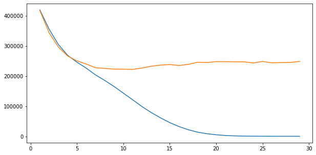
- max_depth가 11일때 가장 낮은 MAE값을 얻을 수 있다.
댓글남기기